02. It's Really Easy! Red Shader! Red Shader


New HLSL in this chapter
- float4: a vector data type with 4 components
- float4x4: 4 X 4 matrix data type
- mul(): multiplication built-in function. Can handle almost all data types
- POSITION: Semantic for vertex position. Useful to read only the position info from vertex data
New math in this chapter
- 3D space transformation: uses matrix multiplication
In the previous chapter, we defined shaders as functions that calculate the positions and colors of pixels. Then, we should try to write a shader that actually does the job, right? We are going to write a very simple shader here so that even readers with no shader programming experience can follow easily. What about a shader that draws a red sphere? [1] We are going to use RenderMoney for this and it will be your first time seeing any HLSL syntax. Yay! Excited? Once you write a shader in RenderMonkey, you can export it to a .FX file, which can be loaded directly into the DirectX framework we prepared in the last chapter.
Initial Step-by-Step Setup
Please follow these steps in order to start writing this shader
- Launch RenderMonkey. A quick scary-looking monkey will welcome you for a moment, and there will be an empty workspace.
- Inside Workspace panel, click the right mouse button on Effect. You will see a pop-up menu.
- From the pop-up menu, select Add Default Effect > DirectX > DirectX, in order. Can you see a red sphere in the preview window?
- You will also see a new shader named Deafult_DirectX_Effect in Workspace panel. Change the name to ColorShader.
Now the screen should look like Figure 2.1.
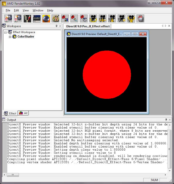
Figure 2.1 Our RenderMonkey project after initial setup
Vertex Shader
Now, click on the plus(+) sign right next to ColorShader. Can you see Pass 0 at the very bottom? Again, click on the plus sign next to it and double-click on Vertex Shader. You will see the code for vertex shader in the shader editor window on the right. Well, this code is actually what we want: it draws a red ball! But we really need to practice, so let's just delete all the code in it.
Did you delete the code? If so, let's get it started! plays music First, I'll show you the full source code for vertex shader below, and explain it line by line after.
struct VS_INPUT
{
 float4 mPosition : POSITION;
};

struct VS_OUTPUT
{
 float4 mPosition : POSITION;
};

float4x4 gWorldMatrix;
float4x4 gViewMatrix;
float4x4 gProjectionMatrix;

VS_OUTPUT vs_main( VS_INPUT Input )
{
 VS_OUTPUT Output;

 Output.mPosition = mul( Input.mPosition, gWorldMatrix );
 Output.mPosition = mul( Output.mPosition, gViewMatrix );
 Output.mPosition = mul( Output.mPosition, gProjectionMatrix );

 return Output;
}
Global Variables vs Vertex Data
There are two types of input values for shaders: global variables and vertex data. Where to put your input values between these two totally depends on whether all vertices in a mesh can use a same value or not. If a same value is used, you should pass it through a global variable. Otherwise, you cannot use a global variable: you have to pass it as part of the vertex data. (i.e. vertex buffer). [2]
Good candidates for global variables include world matrix and camera position. On the other hand, the position and UV coordinates of each vertex are good examples of vertex data.
Input Data to Vertex Shader
First, we are going to declare vertex input data as VS_INPUT structure.
struct VS_INPUT
{
  float4 mPosition : POSITION;
};
Do you remember that the most important role of a vertex shader is transforming each vertex's position from one space to another? It was mentioned in Chapter 1: What is Shader. To do so, you need the vertex position as your input. That is why the above structure retrieves the vertex position via the member variable, mPosition. The reason why this variable is able to retrieve the position info from a vertex buffer is because of POSITION semantic.[3]Often a vertex buffer contains many different data, such as the position, UV coordinates and normal vector, for each vertex. Semantics help you to extract only attributes that are meaningful to you.
So when you see float4 mPosition : POSITION;, it is actually an order to your graphics hardware saying “extract the position information from my vertex data and assign it to mPosition!”
Oh, right. I almost forgot. Then what is float4? This is the variable's data type. float4, a built-in type supported by HLSL, is nothing more than a vector that has four components: x, y, z and w. Of course, each component is a floating-point type as the type name suggests. HLSL also supports other data types, such as float, float2, float3. [4]
Output Data from Vertex Shader
Now that the input data for vertex shader is declared, we need to turn our eyes to output data. When something goes in, something else should come out, right? Do you still remember the super simplified diagram of a GPU pipeline from Chapter 1? In that picture, vertex shader had to output transformed vertex positions so that rasterizer can figure out each pixel's position from them. A key point here: a vertex shader must return a transformed vertex position! Okay, that was enough nagging. Now let's declare the output data as a structure named VS_OUTPUT.
struct VS_OUTPUT
{
  float4 mPosition : POSITION;
};
It looks very familiar, right? We are returning the position data as float4 type. How do you(and your GPU) know its position? You see the semantic, POSITION? Yes! That's how.
Global Variables
We need to declare a number of global variables that will be used in the vertex shader, but doing so without understanding what space transformation is sounds dumb to me.
3D Space Transformation
I said that we need to transform vertex positions into different spaces to draw a 3D object on the monitor. Then, what kind of spaces should we go through to show it? Do you like apples? Let's use an apple as an example.
Object Space
Let's assume we have an apple in our left hand. The center of the apple is the origin point and from this point we can make 3 axes: one to the right direction (+x), one to the up direction (+y), and the other to the forward direction (+z). If you measure every single points on the surface of the apple, you can represent each points in (x, y, z) coordinates, right? Now you group every 3 points to build triangles. The result is an apple model!
Now we move the arm here and there while holding the apple. Even if the hand's position is different, the distance from the origin to each points on the surface of the apple is same, right? This is the object space, or local space. In the object space, every objects (3D models) has its own coordinate system. If you think about it, it's kind of neat. But if you want to handle different objects in a same manner, it's a bit challenging because everyone has its own space! That is where the world space comes in.
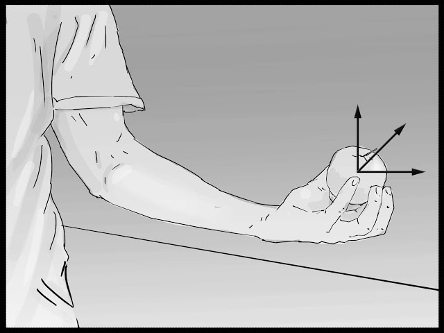
Figure 2.2 An example of object space
World Space
Now why don't you leave the apple right next to your monitor? The monitor is also an object, so it should have its own object space, too. Now we want to handle these two objects in a same manner. So what should we do? It's simple. We just need to bring those two objects into a same space. To do so, we need to make a new space. Do you have a door in the room you are in now? (I really hope you do! :-P ) Let's put an origin at the door and build 3 axes, +x, +y and +z, to right, up and forward directions, respectively. Now, from this origin, can you build new (x, y, z) coordinates for each vertices on the surface of the monitor? You should be able to do the same with the apple, too. We can call this space the world space.

Figure 2.3 An example of world space
####View Space Now, bring out your camera and take two pictures. Make sure the first picture has all these two objects in it, and the second picture doesn't have any of those in it. These two pictures are totally different, right? In the first space, you can see the objects, while you can't at all in the second picture. It means that there got to be positional difference, but positions of the objects in the world space didn't change at all. A-ha! The camera must be using another space! We call this space view space. The origin of the view space is at the center of camera lens, and you can again make 3 axes to the right, up and forward directions.

Figure 2.4 An example of view space. Objects are inside of the camera's view
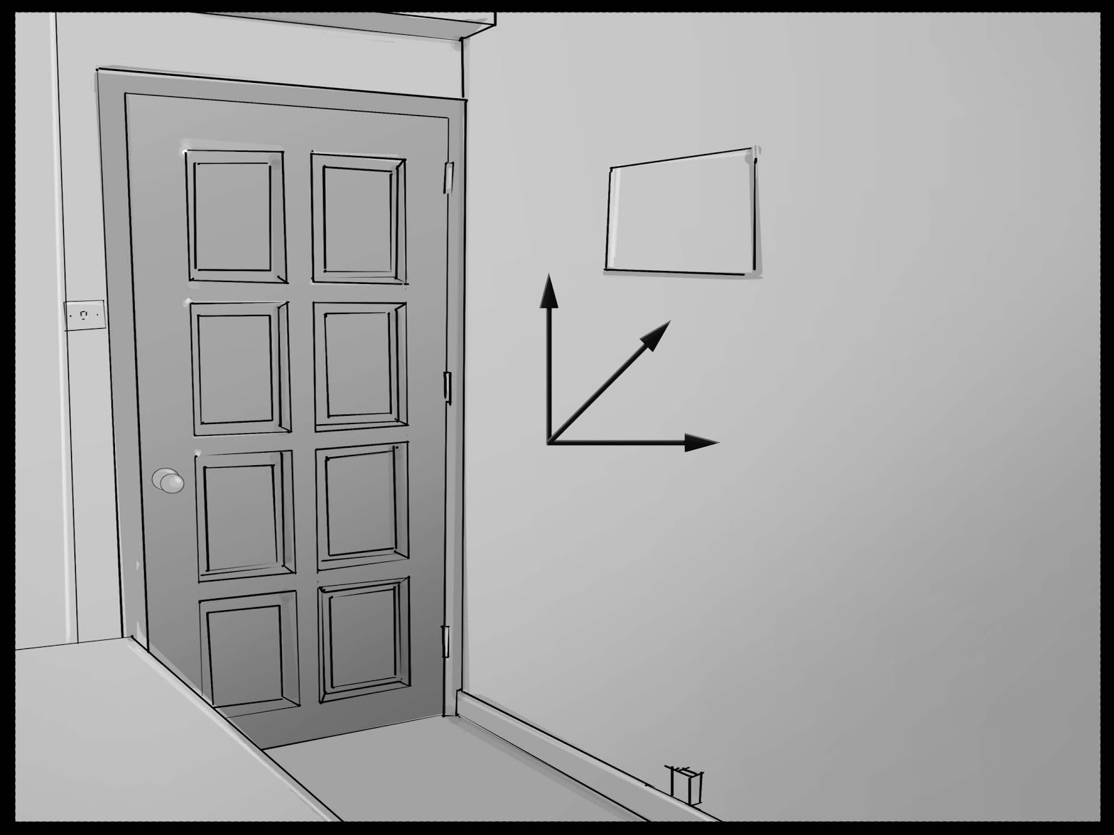
Figure 2.5 An example of view space. Objects are outside of camera's view.
Projection Space
When you see a picture that's taken by your everyday cameras, far-away objects look smaller than ones close by the lens. Just like how you see the world through your eyes. Do you know why our eyes work this way? It's because we humans have a field of view of roughly 100 degree horizontally and 75 degrees vertically. So you get to see more stuff as the distance increases but you are squeezing the “more stuff” into your fixed-size retinas. Your everyday camera does exactly same thing, but there is a special type of cameras called orthogonal cameras. These cameras don't have field of views: instead, they always look straight forward. So if you use these cameras, you can get the consistent object sizes regardless of the distance.
Well, then we should be able to break down these photo-taking steps into two. First step is transforming objects from the world space to the camera space by applying scale, rotation and translation. Second step is projecting these objects onto a 2D image. (i.e., retina in the previous example) So can you distinguish the spaces we used for each of these two steps? Yes, they are view and projection spaces, respectively. With this separation, your view space is independent from the types of projections, such as orthogonal and perspective projections, you are using.
Once you apply the final projection transformation, the transformed result is the final image shown on the screen.
Summary
A usual way of transforming a vertex's space in 3D graphics is matrix multiplication. The number of spaces that an object goes through in order to be displayed on the screen is three: world, view and projection spaces. So you need three matrices, as well. By the way, if you know any space's origin and three axes, you can easily make a matrix that represents that space. [5]
K, now let's sum it up. These are the space transformations that an object is going through:
Object --------> World --------> View ------> Projection
   ⅹWorld Mat   ⅹView Matrix  ⅹProjection Matrix
Since all these matrices are uniform for all the vertices in an object, global variables should be used.
Global Variable Declarations
Now you should have a very clear idea which global variables are needed, right? We need world, view and projection matrices in order to transform vertices. Let's insert add the following three lines in the vertex shader code.
float4x4 gWorldMatrix;
float4x4 gViewMatrix;
float4x4 gProjectionMatrix;
Hey, this is something new! float4x4! This is another data type supported by HLSL. It's very straight forward, right? Yup, this represents a 4 X 4 matrix. As you can guess, there are also similar data types like float2x2 and float3x3.
Now we have these matrices declared. But, who is in charge of passing the values to these variables? Usually the graphics engine in a game takes care of this. But we are using RenderMonkey, so we should follow this monkey's rule. RenderMonkey uses something called variable semantics to pass values to global variables.
Please follow these steps to set the values to the globals:
- In Workspace panel, find ColorShader and right-click on it.
- From the pop-up menu, select Add Variable > Matrix > Float(4x4) in order. It will add a new variable named f4x4Matrix.
- Change this variable's name to gWorldMatrix.
- Now, right-click on gWorldMatrix to select Variable Semantic > World. This is how you pass a value to a variable in RenderMonkey.
- Repeat above steps to make view and projection matrices too. Name the variables as gViewMatrixand and gProjectionMatrix, respectively. Also don't forget to assign variables semantics of View and Projection.
- Lastly, delete matViewProjection variable. This was added by default when we were adding the effect. We do not need this now because we are use gViewMatrix and gProjectionMatrix, instead.
If you finished all the above steps, your Workspace should look like Figure 2.6:
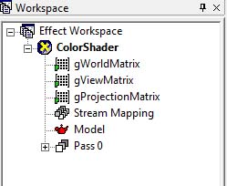
Figure 2.6 Workspace panel after assigning variable semantics
Vertex Shader Function
Finally, all prep works are done. It's time to write the vertex shader function! First up! The function header!
VS_OUTPUT vs_main( VS_INPUT Input )
{
What the function header means are:
- This function's name is vs_main.
- The name of the input parameter is Input and its type is VS_INPUT structure.
- The return type of this function is VS_OUPUT structure.
This is not different from how you define a function in C, right? As mentioned before, HLSL uses a C-like syntax. Now, let's look at the next line.
VS_OUTPUT Output;
This is nothing more than declaring a variable of VS_OUTPUT type that we are going to return at the end of the function. Do you remember what the member of VS_OUTPUT structure was? There was only one member: mPosition, which is in the projection space. That means we are finally apply space transformations! First, we transform the object-space position, stored in Input.mPosition, to the world space. How do you transform a vertex? Yes! You multiply a matrix to it. Since the position vector is a float4, we should multiply a float4x4 matrix, right? Wait. You don't need to flip through your math book to find a way to do this. HLSL already provides an almighty built-in mul() function that can multiply so many different types together. So, you can simply transform the position by calling this function like below:
Output.mPosition = mul( Input.mPosition, gWorldMatrix );
Above code multiplies the world matrix, gWorldMatrix, to an object-space vertex position, Input.mPosition, and assign the result, which is the world-space position, to Output.mPosition. And you do almost exactly same thing to transform the position into the view and projection spaces.
 Output.mPosition = mul( Output.mPosition, gViewMatrix );
 Output.mPosition = mul( Output.mPosition, gProjectionMatrix );
Nothing complicated, right? Then what do we need to do now? Well, the most important role of a vertex shader is transforming a vertex's position, which is originally in the object-space, to the projection space…. Um…. I think we just did it, right? Then, let's just return the result to finish this vertex shader section.
 return Output;
}
Take a moment and press F5 key to compile the vertex shader. You see a red sphere, right? This means we finished the vertex shader section with a great success! If you see any compiler error, please review the code again to see if there is any mistake.
Tip: Got a Shader Compile Error?
If RenderMonkey fails at compiling your code because of typo or invalid syntax, you will see the error messages in the preview window. To see the details about the error, take a look at the output window at the very bottom of RenderMonkey. It should display detailed error messages as well as exact line and column numbers of where the problems are.
Pixel Shader
Now it's time to write the pixel shader. As we did in the Vertex Shader section, find Workspace window and double-click on Pixel Shader. Now, please delete all the code in it. You should type code with your fingers to learn how to code, so please delete all the code in it.
Let's take a look at the full source code, which is only 4-lines long, and then I'll explain it line by line.
float4 ps_main() : COLOR
{
 return float4( 1.0f, 0.0f, 0.0f, 1.0f );
}
The most important role of a pixel shader is returning a color value and we want to draw a red sphere in this chapter. So we can just return red here. But, here's a question: how do you represent red in RGB values? If you are thinking RGB(255, 0, 0), you need to read the following section before writing any pixel shader code.
How to Represent a Color
The reason why most beginners think (255, 0, 0) for the RGB values of the red color is because we are so used to a 8-bit-per-channel format to store an image. An 8-bit integer can represent 256 distinct values. (2^8 = 256) So if you start from 0, you can make 256 integer numbers ranging from 0 to 255. Then, what happens if 5 bits are used per channel instead of 8? 2^5 equals to 32, so 31 will be the maximum value this time. This means that the red color is (255, 0, 0) in a 8-bit format, while it is (31, 0, 0) in a 5-bit format. What a bummer!
So now we know what the problem is. Then, is there any way to represent colors uniformly regardless how many bits are used per channel? If you have played with HDR images in an image editing software, such as Adobe Photoshop, you probably know the answer already. Yes. You can use percentage (%) notation. With this notation, the RGB values of the red color always become (100%, 0%, 0%). This is how shaders represent colors, too. Well almost. You know 0~100% is same as 0.0~1.0 right? So, shaders represent this color as RGB (1.0, 0.0, 0.0).
Pixel Shader Function
Now we know what RGB values need to be output from the pixel shader. So let's write the function now. First is the function header:
float4 ps_main() : COLOR
{
What this line of code means are:
- the function's name is ps_main
- this function doesn't take any parameters
- this function returns a float4
- the return value will be treated as COLOR
One thing to note here is that float4 is used for the return type instead of float3. 4th component is the alpha channel, which is normally used for transparency effect. [6]
By the way, what did we say we need to do in this function? Oh right, we need to return red. The code should be as simple as this:
 return float4( 1.0f, 0.0f, 0.0f, 1.0f );
}
Two things worth mentioning here:
- a color is encoded in a float4 vector in float4(r, g, b, a) form; and
- the value of the alpha channel is 1.0, or 100%, so the pixel is completely opaque.
Now press the F5 key inside the shader editing window to compile vertex and pixel shaders. You will have to do it twice. Once for the vertex shader, and once for the pixel shader. Then as shown in Figure 2.7, you will see a red sphere in the preview window.
Tip: How to Compile a Shader in RenderMonkey
You need to compile vertex and pixel shaders separately in RenderMonkey. Open up each shaders in the shader editor and press F5. When the preview window is about to open, both shaders get compiled, too.
Figure 2.7 Our very first craft! So bloody red!
It was really simple, right? What if you want to show a blue ball instead of a bloody one? Returning float4(0.0, 0.0, 1.0, 1.0) would do it, right? What about green? What about yellow? Yellow is basically a mix of green and red, so…. Oh well, you should be smart enough to know. So, I will stop bothering you here. :)
Now, make sure to save this RenderMonkey project somewhere safe. Actually, save your RenderMonkey project at the end of every chapter because you will re-use them in the following chapters.
(Optional) DirectX Framework
This is an optional section for readers who want to use shaders in a C++ DirectX framework.
First, make a copy of the framework that we made in Chapter 1: What is Shader into a new directory. The reason why we make a copy of the framework for each chapter is because we will extend this framework for each chapter.
Next, it is time to save the shader and 3D model we used in RenderMonkey into files so that they can be used in the DirectX framework.
- From Workspace panel, find ColorShader and right-click on it.
- From the pop-up menu, select Export > FX Exporter.
- Find the folder where we saved the DirectX framework, and save the shader as ColorShader.fx.
- Again, from Workspace panel, right-click on Model.
- From the pop-up menu, select Save > Geometry Saver.
- Again, find the DirectX framework folder, and save it as Sphere.x.
Okay, now go ahead and open the framework's solution file in Visual C++. We are going to add the following code in ShaderFramework.cpp file.
First, we will #define some constants that will be used for the projection matrix.
#define PI      3.14159265f
// Field of View
#define FOV     (PI/4.0f)
// aspect ratio of screen
#define ASPECT_RATIO (WIN_WIDTH/(float)WIN_HEIGHT)
#define NEAR_PLANE  1
#define FAR_PLANE  10000
Then we declare two pointers that will store Sphere.x and ColorShader.fx files after loading.
// Models
LPD3DXMESH gpSphere = NULL;

// Shaders
LPD3DXEFFECT gpColorShader = NULL;
Don't you think it's time to load the model and shader files now? We will add some code to LoadAssets() function that we left empty in Chapter 1.
 // loading shaders
 gpColorShader = LoadShader("ColorShader.fx");
 if (!gpColorShader)
 {
  return false;
 }

 // loading models
 gpSphere = LoadModel("sphere.x");
 if (!gpSphere)
 {
  return false;
 }
To load files, the above code calls LoadShader() and LoadModel() functions, which were implemented in Chapter 1: What is Shader. If any of these results in a NULL pointer, it returns false, meaning “fail to load.” When this happens, there should be some error messages in the output window of Visual C++, so please take a look.
Whenever you load new resources, don't forget to add code to release D3D resources, too. It is to prevent GPU memory leaks. Go to CleanUp() function and insert the following code right before releasing D3D.
 // release models
 if (gpSphere)
 {
  gpSphere->Release();
  gpSphere = NULL;
 }

 // release shaders
 if (gpColorShader)
 {
  gpColorShader->Release();
  gpColorShader = NULL;
 }
Alright, it's almost done. The last step is drawing the 3D object with our shader. We said we will put 3D drawing code inside RenderScene() function, right? Let's go to RenderScene() function.
// draw 3D objects and so on
void RenderScene()
{
Do you remember we used some global variables in the shader? RenderMonkey used something called variable semantics to assign the values to these variables, but we don't have that luxury in our framework. Instead, we have to construct those values and manually pass them to the shader. K, construction time! View matrix is first!
 // make the view matrix
 D3DXMATRIXA16 matView;
 D3DXVECTOR3 vEyePt(0.0f, 0.0f, -200.0f);
 D3DXVECTOR3 vLookatPt(0.0f, 0.0f, 0.0f);
 D3DXVECTOR3 vUpVec(0.0f, 1.0f, 0.0f);
 D3DXMatrixLookAtLH(&matView, &vEyePt, &vLookatPt, &vUpVec);
As shown in the above code snippet, a view matrix can be constructed with D3DXMatrixLookAtLH() function once we have these three information:
- The position of a camera,
- The position where the camera is looking at, and
- The upward direction of the camera. (also known as the up vector)
In this chapter, we assume the camera's current position is at (0, 0, -200) and is looking at the origin (0, 0, 0). In a real game, you would retrieve these information from your camera class.
Next is the projection matrix. Depending on projection techniques being used, we need to call different functions with different parameters. Remember there are two different projection techniques? Yes, perspective and orthogonal. We will use perspective projection here, so the function of choice is D3DXMatrixPerspectiveFOVLH(). [7]
 // projection matrix
 D3DXMATRIXA16   matProjection;
 D3DXMatrixPerspectiveFovLH(&matProjection, FOV, ASPECT_RATIO, NEAR_PLANE, FAR_PLANE);
Yay! One more matrix to go! World Matrix! A world matrix is combination of the following three properties of an object:
- position,
- orientation, and
- scale
What this means is that each object should have its own world matrix. For this example, we assume the object is at the origin (0, 0, 0) without any rotation or scale, so we will just leave our matrix as an identity matrix.
 // world matrix
 D3DXMATRIXA16 matWorld;
 D3DXMatrixIdentity(&matWorld);
Now that we constructed all three global variables, we can pass these values to the shader. You can do this very easily by using the shader class' SetMatrix() function. First parameter of SetMatrix() function is the name of variable in the shader, and the second is a D3DXMATRIXA16 variable declared above in the framework.
 // set shader global variables
 gpColorShader->SetMatrix("gWorldMatrix", &matWorld);
 gpColorShader->SetMatrix("gViewMatrix", &matView);
 gpColorShader->SetMatrix("gProjectionMatrix", &matProjection);
Once all necessary values are passed to the shader, it is time to order the GPU: “Use this shader for anything being drawn from now on!” To give this order, use Begin() / BeginPass() and EndPass() / End() functions. Any meshes drawn between BeginPass() and EndPass() calls will use the shader. Let's look at the below code first.
 // start a shader
 UINT numPasses = 0;
 gpColorShader->Begin(&numPasses, NULL);
 {
  for (UINT i = 0; i < numPasses; ++i)
  {
   gpColorShader->BeginPass(i);
   {
    // draw a sphere
    gpSphere->DrawSubset(0);
   }
   gpColorShader->EndPass();
  }
 }
 gpColorShader->End();
Do you see DrawSubset() call which is wrapped by BeginPass() and EndPass() calls, which are again wrapped by Begin() and End() calls? This will make the GPU to draw gpSphere object with gpColorShader shader.
Some readers might wonder “Why is there BeginPass() function call after Begin()? What is a pass?” Confusing, right? Well, here's a good news; you do not need to worry about it. Passes are only useful when you draw a same object multiple times at once, but we barely do this in real world, so let's just ignore it for now. Just remember that the address of numPasses variable is passed to Begin() function to get the number of passes that exist in the shader. Most of the time, the number is 1. If there are two or more passes in the shader, that means there are more than one vertex/pixel shader pairs, too. So you just need to call BeginPass() / EndPass() as many times as the number of passes.
Now, compile and run the program. You will see the exact same red sphere that you saw in RenderMonkey.
Summary
A quick summary of what we learned in this chapter:
- Per-vertex data is passed as member variables in vertex data.
- Shared data between all vertices is passed as global variables.
- HLSL provides vector-operation-friendly data types, such as float4 and float4x4.
- When transforming vertices into different spaces, matrices are used. To multiply a matrix to a vector, use HLSL intrinsic function, mul().
- HLSL represents a color in a normalized form. [0 ~ 1]
What we learned here is the basics of basics. So unless you can write this simple shader effortlessly, you shouldn't attempt to write other shaders. While I was teaching at a college, I saw some students who did not bother to write this red shader because they thought it was too easy, but later they had hard times with other shaders. It was not because the other shaders were hard, but because those students failed to learn very basic HLSL syntax with this red shader. Therefore, please take your time to write this simple shader once or twice before moving to the next chapter.
Footnotes:
- You will be surprised to see how often graphics programmers use this one-color shader for debugging purposes.
- Not entirely true. Textures can be used for this, too.
- What the heck is a semantic? Just think it as a tag.
- By the way, GPUs are optimized to handle floating-pointing vectors. So, don't worry about using floats over ints. floats are often faster than ints on GPUs.
- For more details on how to manually construct these matrices, please refer to your 3D math book.
- If this value is 1, the pixel is opaque, and 0 means the pixel is completely transparent.
- Please use D3DXMatrixOrthoLH() for orthogonal projection.